![]()
Excel has become, on its own merits, the best application to create spreadsheets of any kind, from those that allow us to carry out day-to-day accounting to database related spreadsheets, in addition to allowing us to represent the data they include in graphs.
All the drop down lists and the dynamic tables that Excel allows us to create, are two of the functions with which we can get the most out of it, the latter being one of the most powerful functions offered by this application that is within Office 365.
What are pivot tables
It is likely that on more than one occasion you have heard of pivot tables, one of the more practical and powerful functions that Excel offers us and it allows us to manage large amounts of data very quickly and easily.
The dynamic tables that we can create with Excel, not only allows us to extract the data from tables, but also allows us extract data from databases created with Access, Microsoft's application for creating databases.
Ok, but what are pivot tables? Pivot tables are filters that we can apply to databases and that also allows us to carry out summations of the results. If you regularly use filters in your spreadsheets, if you use pivot tables, you will see how the time you interact with them is reduced.
How to create pivot tables
To create pivot tables, we need a data source, data source that can be the spreadsheet that we usually use to store the data. If we use a database created in Access, we can set the data source to the table where all the records are stored.
If the data source is a text fileWith the data separated by commas, we can create from that file a spreadsheet from which to extract the data to create the pivot tables. If this type of flat file is the only source of files that we have to create dynamic tables, we should see the possibility of being able to extract the data in another format or create a macro that automatically takes care of creating the dynamic tables every time we import the data.
Although its name may imply complexity, nothing is further from the truth. Create pivot tables it is a very simple process, if we follow all the steps that we indicate below.
Format data source
Once we have the database created, we have to format it so that Excel be able to recognize which are the cells that contain data and which are the cells that contain the names of the records that we want to filter to create the dynamic tables.
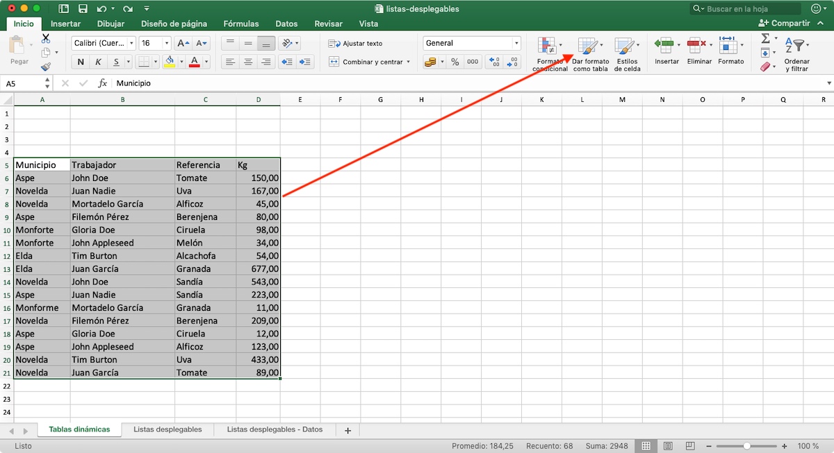
To format a table, the first thing to do is select all the cells that are part of the table and click on the button Format as a table located on the Home ribbon.
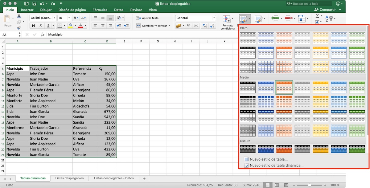
Different layouts will be shown below, layouts that not only modify the aesthetics of the table, but tell Excel that it is a potential data source. In that section, it does not matter which option we select. To the question Where is the data in the table? We must check the box The list contains headers.
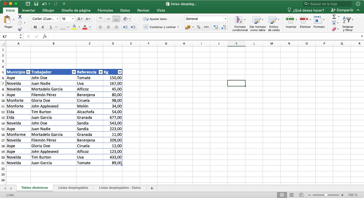
In this way, we indicate to Excel that the first row of the table represents the name of the data in the table, in order to create the dynamic tables, which will allow us to apply automated filters. Once we have the table with the data, and we have formatted it correctly, we can create the dynamic tables.
Create pivot tables
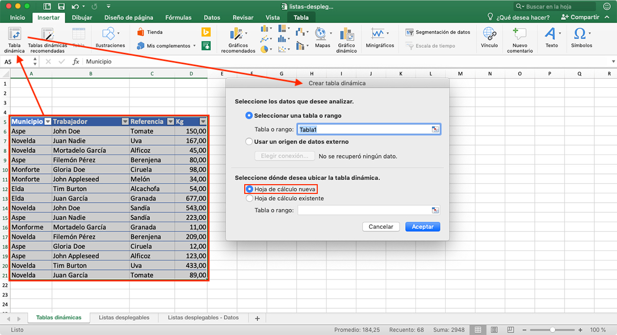
- The first thing we must do is select table where are the data that will be part of the dynamic table, including the cells that show us what type of data they include (in our case Municipality, Worker, Reference, Kg).
- Next, we go to the ribbon and click on Insert.
- Inside Insert, click on Dynamic table and a dialog box named Create pivot table.
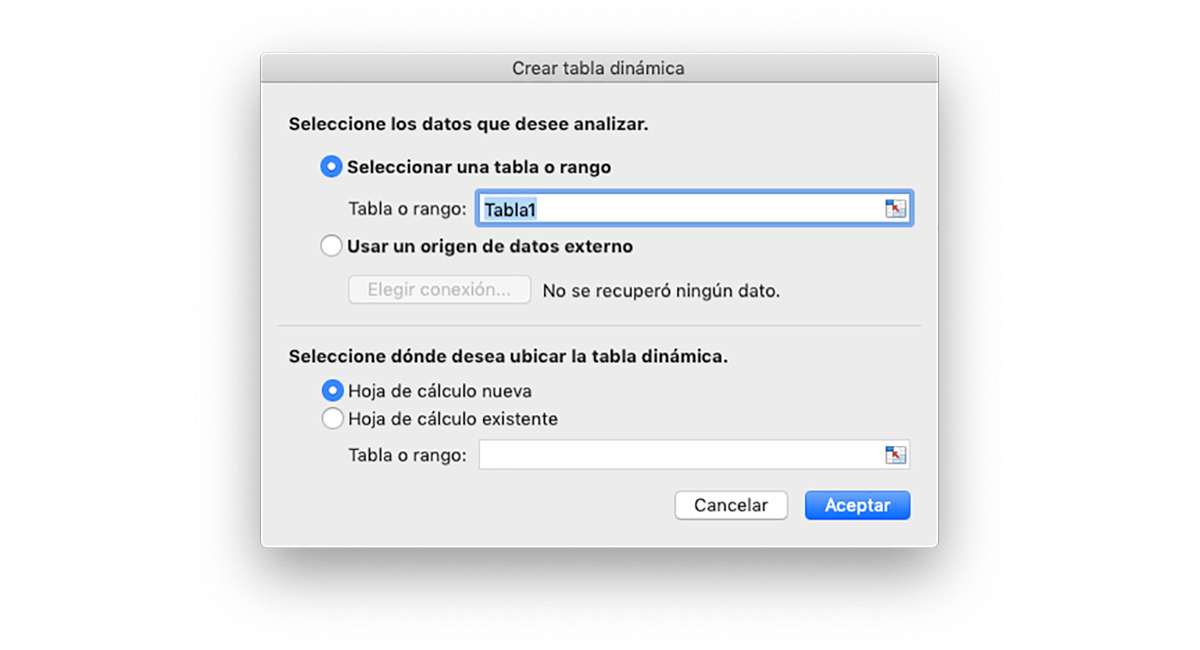
- Within this dialog box we find two options:
- Select the data you want to analyze. As we have selected the table that we wanted to use to create the dynamic table, it is already shown selected under the name Table1. We can change this name in case we intend to add more tables in the same spreadsheet.
- Select where you want to place the pivot table. If we do not want to mix the source data with the pivot table, it is advisable to create a new spreadsheet, which we can call Pivot Table, so as not to confuse with the sheet where the data is displayed, which we can call Data.
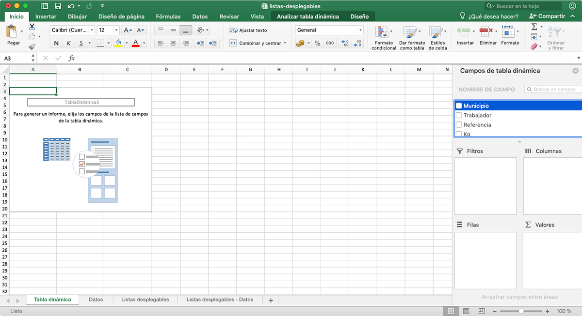
If we have done all the steps, the result should be similar to the one in the image above. If not, you should go through all the steps again. In the panel on the right (panel that we can move through the application or leave it floating) the data that we have selected is shown to which we have to apply the filters we need.
The parameters that we can configure are the following:
Filter

Here we place (by dragging the fields located above) the fields that we want to show that reflect a quantity or a sum. In the case of the example, I have placed the fields Municipality, Worker and Reference to be able to select the total number of references have been sold together (Municipality, Worker and Reference) or by Municipalities, Workers or References.
Within Values, we have included the summation of all references that have been sold. In the case of the example, 6 represents the number of references that all the workers of all the references in the municipality of Novelda have sold.
Columns
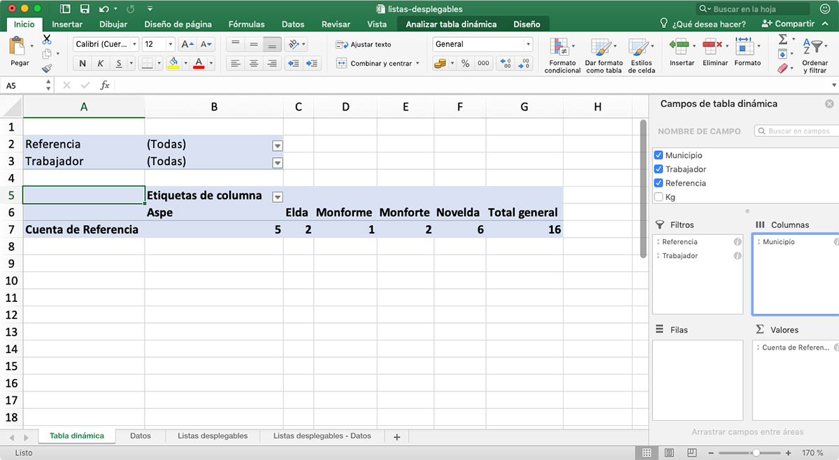
In this section, we must place all the fields that we want to displayed in a drop-down column format to select and display all results related to that value.
In the case of the example, we have placed the Municipality field in Columns, so that it shows us the sum of the number of references that have been sold in all municipalities. If we use the filters, located above, we can further filter the results, establishing the exact reference sold and which worker has sold them.
Rows
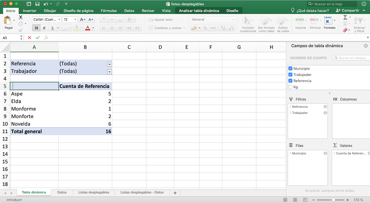
The Rows section allows us to establish which are the values that displayed by rows and the function is the same as with the columns but changing the orientation. As we can see in the image above, when placing the Municipality field in Files, the search results are shown in rows and not in columns.
Values
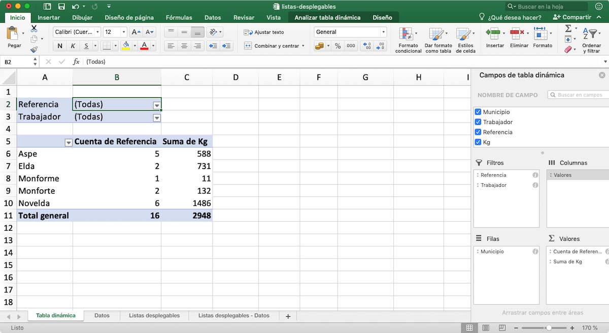
In this section we must add the fields that we want us to show totals. When dragging the Kg field to the Values section, a column is automatically created where the total kg that have been sold by towns are displayed, which is the Row filter that we have added.
Within this section, we also have Reference Account. It is configured to display a count of cities or products. The Sum of KG field is configured so that show total Kg. To modify what action we want to perform at home in one of the established fields, we must click on the (i) located to the right of the field.
Practical tip
If you've made it this far, you might think pivot tables is a very complex world not worth touching. Quite the contrary, how you may have seen in this article, everything is a matter of testing, testing and testing until we can display the data as we want it to be displayed.
If you add a field in a section that you don't want, you just have to drag it out of the sheet so that it is removed. Pivot tables are intended for large amounts of data, not for tables of 10 0 20 records. For these cases, we can make use of the filters directly.